
(Part 1) Compositional Inverse and Power Projection
(Part 2) Composition Algorithm via Transposition Principle (Here)
- Overview
- Transposed mapping and Transposition Principle
- Tranposition of Power Projection and Composition
- Transposed Power Projection Algorithm (Overview)
- Transposed Power Projection Algorithm (Sample Implementation)
- Transposition of Convolution (middle product)
- Transposition of Fourier Transform
- Sample Code of Composition
Overview
When $f(x), g(x)$ are formal power series (FPS), the composite $f(g(x)) = \sum_{i=0}^{\infty}([x^i]f)g(x)^i$ is defined under one of the following conditions:
- $f$ is a polynomial.
- $[x^0]g=0$.
In this article, we introduce an algorithm and an efficient implementation to compute the terms of $f(g(x))$ of degree at most $n-1$, given the terms of $f(x)$ and $g(x)$ up to degree $n-1$, in $\Theta(n\log^2n)$ time.
In simple terms, the previously explained Power Projection can be regarded as a transposed version of the composition problem. Hence, the composition algorithm can be derived by transposing the Power Projection algorithm. Therefore, if you are familiar with the transposition principle, you should be able to derive all the content of this article by yourself.
Considering that many readers of this article may not have learned about the transposition principle or applied it in algorithm derivation, I aimed to provide an explanation that enables learning the transpose principle through the derivation of the composition algorithm.
Furthermore, in the paper “Power Series Composition in Near-Linear Time“, essentially the same composition algorithm discussed in this article is explained without using the transpose principle. So, it would be beneficial to refer to that paper as well for a comprehensive understanding.
Reference
Transposed mapping and Transposition Principle
Even if you don’t fully understand the definition of transposed mappings, I intend to explain the derivation of the composite algorithm in a way that you can understand, so feel free to skip it if it seems difficult.
A brief explanation of transposed mappings is that they are “those that become transposed matrices when written in matrix form.” However, since I am not good at representing mappings with matrices, I will briefly explain it in terms of linear transformations.
Transposed mapping (Abstract Definition, Skippable)
Let $K$ be a ring, $M, N$ be free $K$-modules, and $F\colon M\longrightarrow N$ be a $K$-linear map. Then, the $K$-linear map $F^{T}\colon \mathrm{Hom}_K(N, K) \longrightarrow \mathrm{Hom}_K(M, K)$ is defined by $\phi\mapsto \phi\circ F$. This is called the transposed mapping of $F$.
Transposed mapping (Definition by Components)
Let $K$ be a ring, and $F\colon K^n\longrightarrow K^m$ be a $K$-linear map. The transposed mapping $F^{T}\colon K^m\longrightarrow K^n$ of $F$ is uniquely defined by the following:
For $(x_1, \ldots, x_m)\in K^m$, let $(g_1, \ldots, g_m) = F(f_1, \ldots, f_n)$. Then, there exists a unique $(y_1, \ldots, y_n)$ such that $\sum_jx_jg_j = \sum_iy_if_i$ holds for any $(f_i)$. We define $F^{T}(x_1, \ldots, x_m)$ as this unique solution.
Therefore, the problem of “computing $F^{T}(x_1, \ldots, x_m)$” can be thought of as “expressing the expression $\sum_j x_jg_j$ as $\sum_i y_if_i$.” It may also be approached as “finding the contribution of each $f_i$ in the expression $\sum_j x_jg_j$.”
Note that although the domains and codomains of $F$ and $F^T$ are interchanged, this is entirely different from an inverse mapping.
Transposition Principle
Roughly speaking, the transposition principle states that the following two problems have algorithms with similar computational complexity:
- Given $f = (f_1, \ldots, f_n)$ as input, compute $F(f) = (g_1, \ldots, g_m)$.
- Given $x=(x_1, \ldots, x_m)$ as input, compute $F^{T}(x) = (y_1, \ldots, y_n)$.
Deriving the algorithm of $F^{T}$ from the algorithm of $F$ should theoretically be possible by enumerating all arithmetic operations of $F$, but it becomes challenging with complex algorithms. In practice, it’s often done by decomposing the algorithm into steps larger than arithmetic operations and solving each step’s transpose problem (sometimes without using the transpose principle). In this article, we derive the composite algorithm using such steps.
Tranposition of Power Projection and Composition
First, let’s explain that “the transposition of Power Projection is composition.”
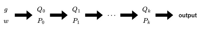
Let’s recap Power Projection. I’ve changed some symbols from the previous article. Also, please assume that all lengths of sequences and FPS are $n$.
[Power Projection] Given a sequence $w=(w_j)$ and an FPS $g(x)$. Compute$\mathrm{PowProj}(w,g)[i] := \sum_{j}w_j[x^j]g(x)^i$ for each $i$.
Now, let’s consider the transpose of this problem. This is not entirely accurate because transposition is defined for linear transformations, but the mapping $(w,g)\mapsto \mathrm{PowProj}(w,g)$ is not a linear transformation.
However, if we fix $g$, the mapping $\mathrm{P}_g = \mathrm{PowProj}(-,g); w\mapsto \mathrm{PowProj}(w,g)$ is a linear transformation. Therefore, we can consider what the transposed mapping $\mathrm{P}_g^T$ of $\mathrm{P}_g$ would be.
Based on the definition by components of transposed mappings, for $f=(f_0,\ldots,f_{n-1})$, $(x_0,\ldots,x_{n-1}) = \mathrm{P}g^T(f)$ is a sequence such that for any $w$, $\sum{j}w_jx_j = \sum_i f_i\mathrm{P}_g(w)[i]$. In other words, the transposed problem of “compute $\mathrm{P}_g(w)$” is formulated as “compute $\mathrm{P}_g^T(f)$” as follows:
[Transposition of Power Projection] Given $f,g$, consider the value $X = \sum_i f_i \mathrm{P}_g(w)[i]$ for a sequence $w$. Determine $(x_0,\ldots,x_{n-1})$ when expressed $X$ as $\sum_{j}w_jx_j$.
Recalling the definition $\mathrm{P}_g(w)=\mathrm{PowProj}(w,g)$,
$$X = \sum_if_i\sum_jw_j[x^j]g(x)^i = \sum_jw_j[x^j]\sum_if_ig(x)^i.$$
Then it’s clear that the solution to this problem is $x_j=[x^j]\sum_if_ig(x)^i=[x^j]f(g(x))$. Hence, it’s evident that there’s a transposed relationship between Power Projection and composition, more precisely, between $w\mapsto \mathrm{PowProj}(w,g)$ with $g$ fixed and $f\mapsto f(g(x))$.
Therefore, according to the transposition principle, we can say that there exists an algorithm for composition with computational complexity similar to that of Power Projection. In the following, let’s explore what this algorithm specifically looks like.
Transposed Power Projection Algorithm (Overview)
Assuming a basic understanding of the Power Projection algorithm, let’s represent it as follows:
The transposed Power Projection problem involves finding the coefficients when expressing $X = \sum_i f_i \mathrm{P}_g(w)[i]$ in terms of $w$, given $f$ and $g$ as inputs. Adding the steps to compute $X$ can make it easier to understand.
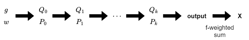
The problem to solve is to “Express $X$ in terms of $w$ given $f$ and $g$.” It’s important to be mindful of what is given and what needs to be determined from the figures above.
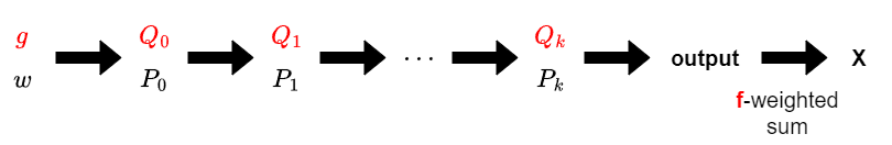
Among the elements in the above diagram, $f$ and $g$ are given, and $Q_i$ can be computed from $g$, so all the quantities in red text can be considered as given. Everything else is calculated sequentially when $w$ is given (more precisely, it’s a calculation based on the linear transformation determined by the “given quantities”).
We solve the transposed problem by following steps:
- Knowing that $X$ is a linear combination of coefficients $f_i$ of the output.
- Using the result of previous step, determine the coefficients when expressing $X$ as a linear combination of elements of $P_k$.
- $\vdots$
- Using the result of previous step, determine the coefficients when expressing $X$ as a linear combination of elements of $P_0$.
- Using the result of previous step, determine the coefficients when expressing $X$ as a linear combination of elements of $w$.
In this manner, we compute the answer in the reverse order of the original problem (corresponding to the property of transposition of matrix products: $(A_1\cdots A_n)^T=A_n^T\cdots A_1^T$).
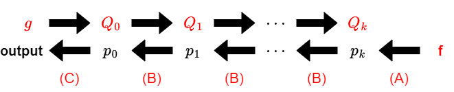
Summarizing what we’ve discussed so far, the overall scheme of the composite algorithm can be represented by the following diagram:
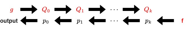
First, we compute $Q_0, Q_1, \cdots$ from $g$. This involves exactly the same calculations as the Power Projection algorithm.
Next, we sequentially determine the coefficients $p_i$ of $X$ when expressed as a linear combination of elements of $P_i$, starting from the end. Repeating this calculation eventually yields the coefficients of $X$ when expressed as a linear combination of elements of $w$, which gives us the desired $f(g(x))$.
Transposed Power Projection Algorithm (Sample Implementation)
To simplify the explanation, let’s assume $[x^0]g=0$ and that $n$ is a power of $2$.
To implement the transposed algorithm, we first prepare the implementation of the original algorithm.
As explained earlier, the computation follows the flow of “computing $Q_i$ iteratively from $g$, and then traversing back based on the results.” Therefore, implementing it using recursion would make the code concise. Additionally, unlike in Power Projection, we’ll need to reuse the values of $Q_i$ even after computing $Q_{i+1}$, so we’ll implement it in a way that avoids overwriting the same array for reuse.
With that in mind, I prepared the following implementation. (If you need information about templates used, please pick it up from the submission).
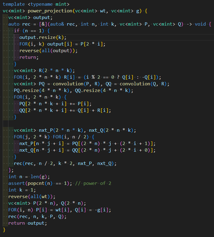
Furthermore, separating the computation into calculations for $Q$ and calculations for $P$ makes it easier to understand.
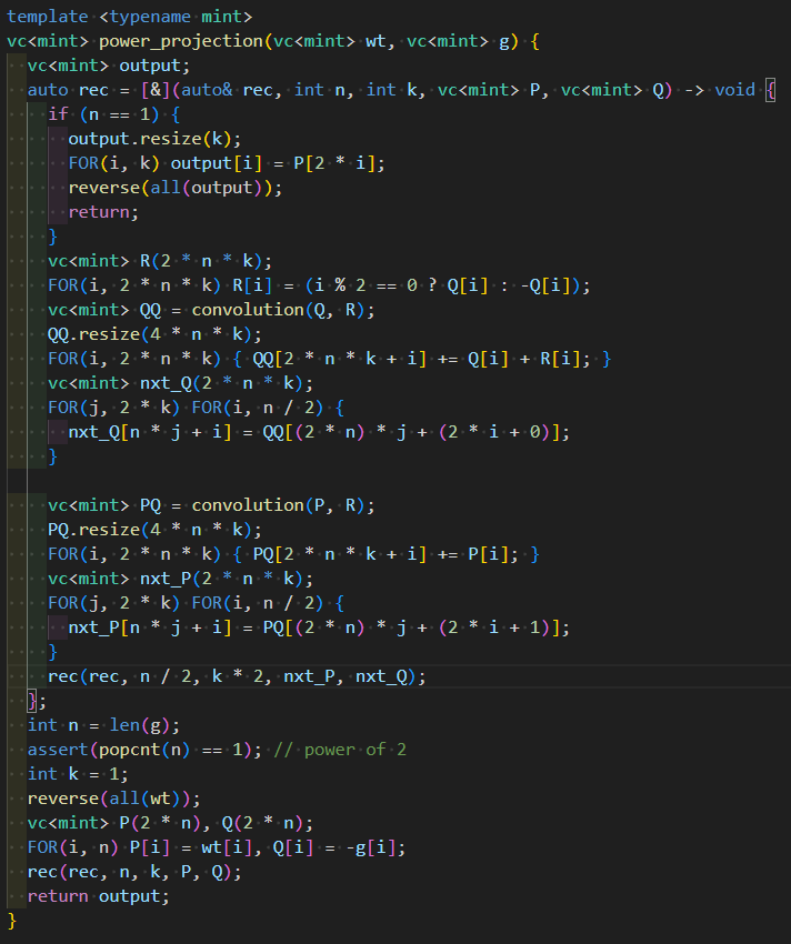
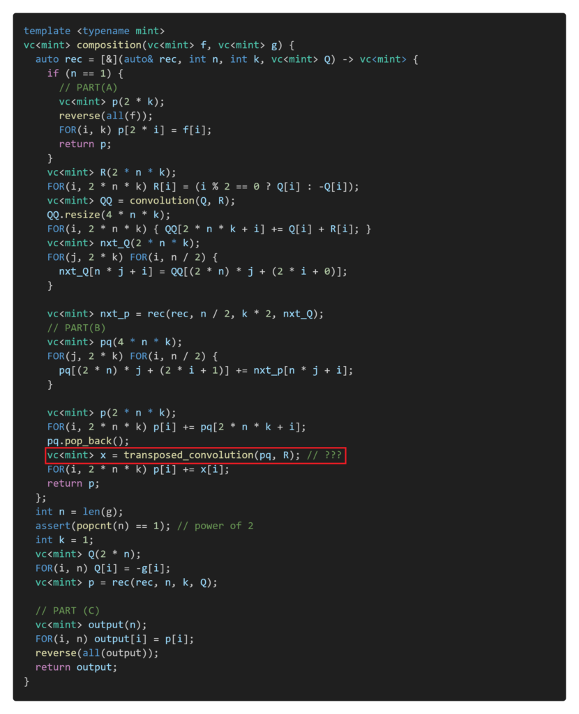
Let’s modify this code to make it an implementation for composition. Instead of implementations like “calculating nxt_P from P,” we’ll replace them with implementations like “calculating coefficients of P from coefficients of nxt_P.” Here’s roughly how the implementation should look:
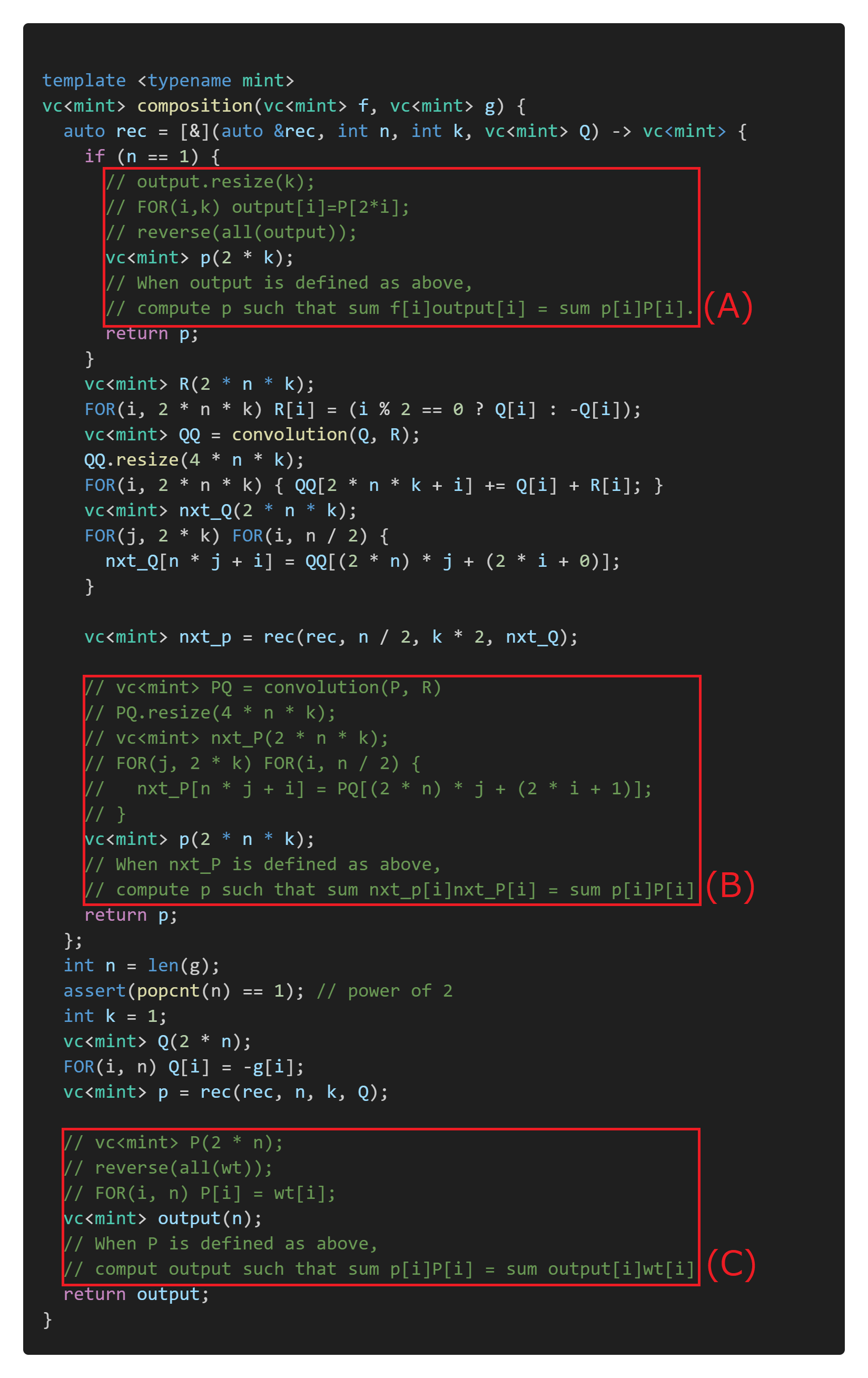
There are three places marked with red boxes, and replacing them with appropriate implementations will complete the implementation for composition. Each of these corresponds to the following parts of the overall algorithm diagram.
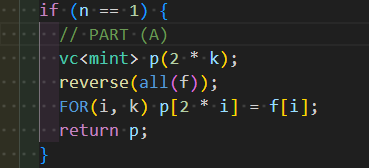
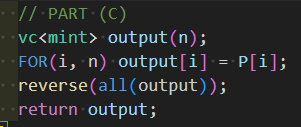
Now, (A) and (C) are straightforward, and if you understand what needs to be calculated correctly, you can implement them quickly. For these parts, which involve simply rearranging elements in arrays to correspond to each other, you just need to reinsert them at the appropriate locations and fill the rest with zeros.
Finally, let’s consider part (B). When you’re not sure what the transpose will look like, it’s helpful to break it down into several steps. Here, it’s implemented in two steps: “determining PQ from P” and “determining nxt_P from PQ”. We’ll implement this by tracing back in reverse order.
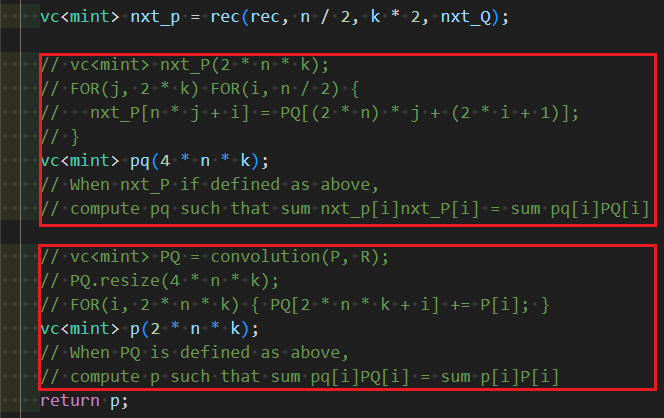
The upper half is straightforward. Let’s focus on the lower half.
The lower half involves transferring pq using the transposed mapping of $\mathrm{convolution}(-, R)$. Let’s leave this part for later. With that, the implementation is completed, excluding the transposition of convolution.
Transposition of Convolution (middle product)
Transposition of Convolution (middle product)
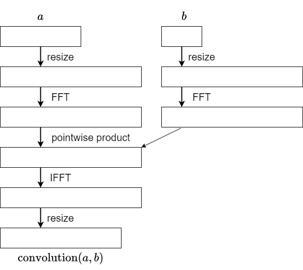
Let $a$ be a sequence of length $n$, and $b$ be a sequence of length $m$. Then, $c = \mathrm{convolution}(a,b)$ is a sequence of length $n+m-1$ defined by $c_k = \sum_{i+j=k}a_ib_j$.
When $b$ is fixed, $\mathrm{convolution}(-,b); a\mapsto \mathrm{convolution}(a,b)$ is a linear mapping that maps a sequence of length $n$ to a sequence of length $n+m-1$. Let’s consider what the transposed mapping of this function looks like.
It’s a mapping that transfers a sequence $x$ of length $n+m-1$ to a sequence $y$ that satisfies $\sum_{k}c_kx_k = \sum_{i}a_iy_i$. Substituting $c_k = \sum_{i+j=k}a_ib_j$, the left-hand side becomes $\sum_{i}\sum_ja_ib_jx_{i+j}=\sum_i a_i(\sum_jb_jx_{i+j})$. Therefore, the transposition problem can be formulated as follows:
Given a sequence $x$ of length $n+m-1$, find the sequence $y$ of length $n$ determined by $y_i=\sum_jb_jx_{i+j}$.
This sequence $y$ is also known as the middle product of $x$ and $b$.
For readers familiar with convolution, they may notice that this can be easily computed using convolution. By convolving one of $b$ or $x$ in reverse order, and then gathering the appropriate values, the output can be obtained. If implemented directly, this would require an FFT of length around $n+2m$.
However, with an appropriately implemented middle product, a faster implementation can be achieved using FFT of length around $n+m-1$. Below, we will explain this in two different way.
(The middle product is often usable beyond the context of transposition problems. Many people may be performing normal convolutions without realizing that the middle product can be utilized.)
Calculating the Middle Product (Derivation 1)
If we reverse $b$, what we want to compute becomes $y_i=\sum_{j}x_{i+j}b_{m-1-j}=\sum_{j+k=m+i-1}x_jb_k$. Therefore, after convolving $x$ and $b$, we only need to extract elements from the $(m-1)$-th to the $(m+n-2)$-th positions.
Exploiting the fact that we only need a small portion after convolution, we can replace the convolution with circular convolution. That is, we choose $L$ satisfying $L\geq n+m-1$, perform circular convolution of length $L$ on $x$ and $b$, then extract elements from the $(m-1)$-th to the $(m+n-2)$-th positions.
Indeed, for $0\leq j < n+m-1$ and $0\leq k<m$, we have $0\leq j+k<n+2m-1\leq L+m$, showing that the terms entering from the $(m−1)$-th to the $(2m+n-2)$-th positions in circular convolution are exactly the terms entering in that range in normal convolution.
Calculating the Middle Product (Derivation 2)
Let’s derive an algorithm from the transposition principle, noting that the middle product is the transposition of convolution.
Convolution can be computed using the following steps:
When considering transposition, please note that $b$ is treated as a constant. The operation of obtaining $\mathrm{convolution}(a,b)$ from $a$ is represented as the composition of five (determined by $b$) linear mappings. The transposed mapping can be expressed as the composition of these five mappings in reverse order.
For the pointwise product, recalling that $b$ is treated as a constant, it is just a component-wise scalar multiplication. Therefore, the transposition follows the same scalar multiplication pattern. Thus, the following implementation is feasible:
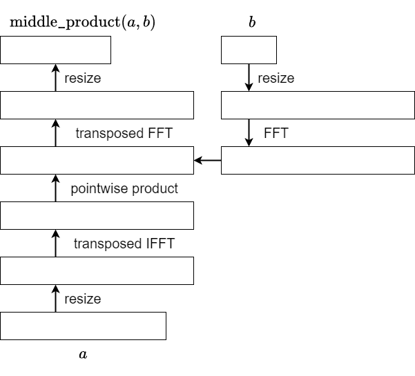
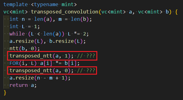
We just need to understand how the transposition of FFT and IFFT works. This is another important issue, not limited to the application in middle product. I will explain this again in the following.
Transposition of Fourier Transform
When $a$ is a sequence of length $n$, and we fix the primitive $n$-th root of unity $\omega$, the Fourier transform of $a$, denoted as $\mathcal{F}[a]$, is defined as:
$$ \mathcal{F}[a]_i = \sum_{j} \omega^{-ij} a_j .$$
The Fourier transform can be regarded as a multiplication by a symmetric matrix, and therefore the transpose of the Fourier transform is simply the Fourier transform itself.
The inverse Fourier transform is defined as:
$$ \mathcal{F}^{-1}[a]_i = \frac{1}{n} \sum_j \omega^{ij} a_j .$$
and it serves as the inverse operation of the Fourier transform. Like the Fourier transform, it can be written by a symmetric matrix, so the transpose of the inverse Fourier transform is the inverse Fourier transform itself.
(Note that there are variations in the definitions of these operations across different references, including differences in scaling factors such as $1/n$ ).
That’s mostly correct, but there’s an important caveat.
Many FFT implementations output sequences arranged in bit-reversed order, including widely-used libraries like the one in the AtCoder Library. Consequently, depending on the FFT implementation, it’s not guaranteed that the FFT operation itself is equal to its transpose.
Transposition of Bit-Reversed FFT
Let $n=2^k$ be a power of $2$, and $\mathrm{rev}(i)$ as the bit-reversal of $i$ up to the $k$th binary digit.
Let’s define bit-reversed FFT and bit-reversed IFFT as follows (though strictly speaking, FFT refers to the algorithm rather than the transformation itself, let’s consider it more broadly here):
- Bit-reversed FFT: Input $a$ and output $b$ defined by $b_i = \sum_j \omega^{-\mathrm{rev}(i)\cdot j}a_j$.
- Bit-reversed IFFT: Input $b$ and output $a$ defined by $a_i = \dfrac{1}{n}\sum_{j} \omega^{i\cdot \mathrm{rev}(j)}b_j$.
Therefore, their transposes can be described as follows:
- Transposed Bit-reversed FFT: Input $b$ and output $a$ defined by $a_i = \sum_j \omega^{-i\cdot \mathrm{rev}(j)}b_j$.
- Tranposed Bit-reversed IFFT: Input $a$ and output $b$ defined by $b_i = \dfrac{1}{n}\sum_j \omega^{\mathrm{rev}(i)\cdot j}a_j$.
Comparing them, you’ll notice that “bit reversed FFT” and “transposed bit reversed IFFT“, as well as “bit reversed IFFT” and “transposed bit reversed FFT“, are nearly identical. The only differences lie in the presence of $\dfrac{1}{n}$ overall and a negative exponent. Therefore, we can conclude the following:
- The transposed bit-reversed FFT is: bit-reversed IFFT, then reversing all but the first element, then scaling it by $n$.
- The transposed bit-reversed IFFT is: reversing all but the first element, then bit-reversed FFT, then scaling it by $1/n$.
The operation of “reversing all but the first element” is to send $i$-th element to $(n-i)$-th position, and since $\omega^{-i} = \omega^{n-i}$, the exponent is negated.
Sample Code of Composition
The implementation of composition is now complete based on the preceding discussions. The following sample code faithfully follows the explanation in this article.
Sample Code(1035ms)https://judge.yosupo.jp/submission/204008
The execution time is approximately the same as the original implementation of Power Projection (Inverse Function, 1042ms). The latter is slightly slower because it computes the formal power series pow after Power Projection.
In this article, for the sake of simplicity, we assumed that $n$ is a power of $2$ and $[x^0]g=0$ in the implementation. So, when integrating it into your library, please pay attention to these points.
In this article, we selected one implementation example of Power Projection and implemented composition using the transposition principle. Of course, starting with a more efficient implementation of Power Projection would yield an even faster implementation of composition. For example, from the implementation introduced in the previous article (Proposal 2), I obtained the following impolementation.
Sample Code(479ms)https://judge.yosupo.jp/submission/204011
Try challenging yourself with the transposition principle as an exercise.