
(Part 1) Compositional Inverse and Power Projection (Here)
(Part 2) Composition Algorithm via Transposition Principle
Japanese Version → FPS 合成・逆関数の解説(1)逆関数と Power Projection
Overview
noshi91 has presented a method to compute the Composition and Compositional Inverse of formal power series in $\Theta(n\log^2 n)$ time.
This method offers a simple algorithm for fundamental problems, improving upon known computational complexity and attracting considerable attention both domestically and internationally.
Subsequently, there have been discussions, utilizing the transposition principle for simpler derivations of the algorithm of Composition (by Elegia, hos_lyric), and algorithms have been implemented with good performance (by Nachia and others). Feeling a lack of articles explaining these matters, I’ve decided to provide some explanation.
I plan to divide the explanation into two parts, (1) and (2). In this article (1), I will cover the Compositional Inverse, and Power Projection used in the implementation of Compositional Inverse. In article (2), I will discuss the derivation and implementations of the Composition algorithm using the transposition principle.
In this article, we assume that convolution of polynomials can be implemented in $\Theta(n\log n)$ time. If you are interested in using it for competitive programming, it is acceptable to consider choosing a prime number $p$ and working with coefficients modulo $p$.
I denote formal power series as FPS. I will use the notation FFT without distinguishing between FFT and NTT (however, in my source code, I use the term NTT).
Reference
- https://noshi91.hatenablog.com/entry/2024/03/16/224034 (noshi91, in Japanese)
- https://arxiv.org/abs/2404.05177 (noshi91, Elegia)
The Composition algorithm is explained without using the transposition principle. - Library Checker We can verify these alrogithms.
- FPS composition f(g(x)) の実装について (Nachia, in Japanese)
Nachia’s notes on the implementations of FPS composition. Nachia achieved the fastest implementation as March 2024 for the problems on Library Checker. - On implementing O(nlog(n)^2) algorithm of FPS composition (hly1024, codeforces blog)
- Why is no one talking about the new fast polynomial composition algorithm? (Kapt, codeforces blog)
Compositional Inverse and Power Projection
Let $f$ be an FPS such that $[x^0]f=0$ and $[x^1]f\neq 0$. It can be proven that there exists a unique FPS $g$ satisfying $g(f(x))=f(g(x))=x$, and it is called the compositional inverse of $f$.
Let $c=[x^1]f$. It is easy to see that if $f(x)/c$ has a compositional inverse $g(x)$, then $g(x/c)$ will be the compositional inverse of $f(x)$. Therefore, the problem of find the compositional inverse can be reduced to the case where $[x^1]f=1$.
In this case, the compositional inverse $g$ satisfies $[x^0]g=0$ and $[x^1]g=1$.
Given the parts of $f$ up to degree $n$, we aim to find the parts of $g$ up to degree $n$. According to the Lagrange inversion formula, for any $i$,
$$n[x^n]f(x)^i = [x^{n-i}]i\cdot (g(x)/x)^{-n}$$
holds. If we can compute the left-hand side for $i=1,\ldots,n$, then we can obtain $(g(x)/x)^{-n}$ up to the degree $n-1$. Taking the $-1/n$ -th power, we can find $g(x)/x$ up to the degree $n-1$ (note that $[x^1]g=1$ is required for defining the $-1/n$ -th power and ensuring it matches $g(x)/x$). Thus $g(x)$ can be computed up to degree $n$.
Ultimately, the problem of finding the compositional inverse can be reduced to the following computation:
Compute $[x^n]f(x)^i$ for $i=1,\ldots,n$.
This is a special case of a problem called Power Projection, which is explained below. The method by noshi91 solves Power Projection in $\Theta(n\log^2 n + m\log m)$ time. Therefore, the problem of finding the compositional inverse can be solved in $\Theta(n\log^2 n)$ time.
Next, we will explain algorithms for solving Power Projection and how to implement it with good performance.
Power Projection Algorithm
Let’s consider the following problem of enumerating a linear combination (projection) of powers of an FPS with some weights:
[Power Projection] Given a sequence $(w_0, \ldots, w_{n-1})$ and an FPS $f(x)$, compute the following for $i=0, \ldots, m-1$: $\sum_{j=0}^{n-1}w_j\cdot [x^j]f(x)^i$.
In this article, for the sake of simplicity, we assume that $n$ is a power of $2$. If necessary, we can reduce it to this case by appending $0$s to the end of $f$ and $w$. (Not only does this simplify the explanation, but it also slightly reduces the number of cases in the implementation without significantly changing the constant factors in computational complexity).
If we consider $g(x)=\sum_{j=0}^{n-1}w_{n-1-j}x^j$ instead of $w_j$, the problem can be rephased as follows:
Given FPS $f(x), g(x)$, compute $[x^{n-1}]g(x)f(x)^i$ for $i=0,\ldots,m-1$.
By considering $2$-variable FPS, we have $g(x)f(x)^i = [y^i]\dfrac{g(x)}{1-yf(x)}$. Therefore, if we let $P(x,y)=g(x)$ and $Q(x,y)=1-yf(x)$, what we want to compute becomes $[x^{n-1}]P(x,y)Q(x,y)^{-1}$.
We compute this by using the same technique as the Bostan-Mori’s algorithm, namely the $Q(x)Q(-x)$ technique (Graeffe’s method).
Assuming that $n$ is a power of $2$ not less than $2$, we utilize the following equation: $$[x^{n-1}] P(x,y)Q(x,y)^{-1} = [x^{n-1}]P(x,y)Q(-x,y)\cdot (Q(x,y)Q(-x,y))^{-1}.$$
The product $Q(x,y)Q(-x,y)$ is an even function of $x$, and there exists some $Q_1(x,y)$ such that $Q(x,y)Q(-x,y)=Q_1(x^2,y)$. If we decompose the part of $P(x,y)Q(-x,y)$ into odd and even degree terms with respect to $x$ as $P(x,y)Q(-x,y) = xP_1(x^2,y)+P_2(x^2,y)$, then we have:
$$[x^{n-1}] P(x,y)Q(x,y)^{-1} = [x^{n-1}]xP_1(x^2,y)Q_1(x^2,y)^{-1} + [x^{n-1}]P_2(x^2,y)Q_1(x^2,y)^{-1}.$$
Given that $n\geq 2$ is a power of $2$, it is clear that $[x^{n-1}]P_2(x^2,y)Q_1(x^2,y)^{-1}$ is equal to $0$. Hence
$$[x^{n-1}] P(x,y)Q(x,y)^{-1} = [x^{n-1}]xP_1(x^2,y)Q_1(x^2,y)^{-1} = [x^{n/2-1}]P_1(x,y)Q_1(x,y)^{-1}.$$
It’s worth noting that for $P_1$ and $Q_1$, we only need to keep terms up to degree $n/2-1$.
This transformation preserves the form of the problem while reducing the size of $n$ by half. By repeating it $\log_2n-1$ times, we can reduce the problem to the case of $n=1$. When $n=1$, we are left with the problem of “Find $p(y)/q(y)$ up to degree $m-1$”, which is simply FPS division. In summary, the following algorithm roughly provides the solution.
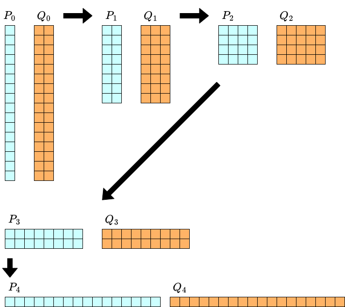
- Let $P_0(x,y)=g(x), Q_0(x,y)=1-yf(x), n_0=n$.
- Define $P_k$ and $Q_k$ as follows, until $n_k=1$.
- Extract $n_k/2$ terms of the odd-degree part with respect to $x$ from $P_k(x,y)Q_k(-x,y)$ and let it be $P_{k+1}(x,y)$.
- Extract $n_k/2$ terms of the even-degree part with respect to $x$ from $Q_k(x,y)Q_k(-x,y)$ and let it be $Q_{k+1}(x,y)$.
- Let $n_{k+1}=n_k/2$.
- When we reach $n_k=1$, $P_k(x,y)Q_k(x,y)^{-1}$ is just a division of $1$-variable FPS. Compute this up to degree $m-1$ and output it.
Furthermore, in the case where $[x^0]f=0$, it always holds that $[x^0]Q_k=1$, and the desired output is simply $P_k(x,y)$. General power projection can be reduced to the case of $[x^0]f=0$ by using equations such as $\sum_j w_j[x^j](f(x)+c)^i=i!\cdot \sum_{p+q=i}\dfrac{w_j}{p!}[x^j]f(x)^p\cdot \dfrac{c^q}{q!}$. Therefore, it may be a good idea to specialize the implementation for the case of $[x^0]f=0$, and reduce to it if neccesary. (The sample code I introduce in this article follow this approach. )
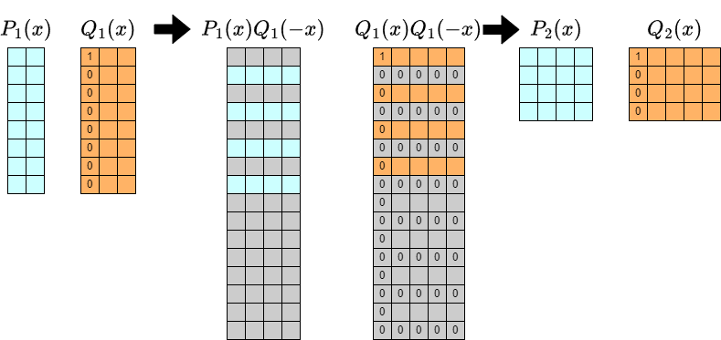
To analyze the computational complexity, let’s consider the degrees of each $P_k$ and $Q_k$. For example, when $n=16$, it looks like the figure below. In this figure, there is a term of $x^iy^j$ in row $i$ and column $j$.
As we proceed with the computation, the degree with respect to $y$ doubles with each iteration. On the other hand, the degree with respect to $x$ halves each time. Therefore, at each stage of the iteration, the number of terms to be retained is always $\Theta(n)$. Multiplication of such two-variable polynomials (2D convolution) can be performed in $\Theta(n\log n)$ time. We need to perform this iteration $\log_2 n$ times and an FPS division up to degree $m-1$. Thus the overall computational complexity becomes $\Theta(n\log^2 n + m\log m)$.
Let’s take a closer look at each iteration of the algorithm described above.
The length of $Q_k$ in the $y$ direction is $2^k+1$, which seems not well-suited for convolution and might worsen the constant factors.
On the other hand, since $Q(x,y)=1-yf(x)$, $[y^0]Q_k$ is always $1$. Therefore, handling the troublesome degree of $Q_k$ can be resolved by properly handling the $[y^0]$-part.
However, handling parts with unified treatment where degree ranges from $[1,2^k]$ might become cumbersome in the implementation. To address this, considering the “reverse” in the $y$ direction could lead to a more concise implementation. Although this is not nesessary for optimization purposes, I’ll include it in this article for ease of understanding.
Let’s make a slight modification to the algorithm.
- Let $P_0(x,y)=g(x), Q_0(x,y)=-f(x)+y, n_0=n$.
- Define $P_k$ and $Q_k$ as follows, until $n_k=1$.
- Extract $n_k/2$ terms of the odd-degree part with respect to $x$ from $P_k(x,y)Q_k(-x,y)$ and let it be $P_{k+1}(x,y)$.
- Extract $n_k/2$ terms of the even-degree part with respect to $x$ from $Q_k(x,y)Q_k(-x,y)$ and let it be $Q_{k+1}(x,y)$.
- Let $n_{k+1}=n_k/2$.
- When we reach $n_k=1$, let $p(y), q(y)$ be the reverses of $P_k(x,y), Q_k(x,y)$ (more formally, $p(y)=y^{n-1}P_k(x,1/y)$ and so on ). Then output $p(y)q(y)^{-1}$ up to degree $m-1$.

Then, at each stage, the highest degree term of $Q_k$ with respect to $y$ becomes the unique term $y^{2^k}$ and the implementations strategy involves convolving the degree range $[0,2^k-1]$ while handling the $2^k$-degree part accordingly.
If you’re not particularly concerned about performance tuning, implementing based on the understanding so far should suffice. While 2D convolution is required, you can easily implement it even without 2D convolution library by reducing it to a one-dimensional convolution, by associating the $(i,j)$-th term of the $2$-variable polynomial with $(2ki+j)$-th term of the $1$-variable polynomial, as demonstrated in the following sample code.
Sample Code(1083ms):https://judge.yosupo.jp/submission/203740
In the above sample code, to make the algorithm’s operations more understandable, we convert the two-dimensional array into a one-dimensional array, perform convolution, and then convert it back to a two-dimensional array. However, it’s also possible to implement everything directly using a one-dimensional array from the begining as the following sample code. While it doesn’t significantly improve execution time, it saves a considerable amount of memory and simplifies the implementation.
Sample Code(1042ms):https://judge.yosupo.jp/submission/203746
Speeding up Power Projection using FFT (Proposal 1)
When polynomial FFT is feasible, it enables better implementations in terms of constant factors. Many acceleration technique are common with the problem:
So, if you’re not familiar with the following discussion, it might be good to tackle the acceleration of this problem first.
The following resource may also be helpful (in Japanese).
Let’sdefine a polynomial of degree $a-1$ with respect to $x$ and degree $b-1$ with respect to $y$ as a polynomial of shape $(a,b)$.
At the beginning of each iteration, let’s assume that $P=P_k$ and $Q=Q_k$ have shapes $(n,m)$. We denote $R(x)=Q(-x)$. We want to extract appropriate parts of $P(x)R(x)$ and $Q(x)R(x)$.
$P(x)R(x)$ and $Q(x)R(x)$ can be computed as follows:
- Extend $P(x),Q(x)$ and $R(x)$ to shape $(2n,2m)$ by zero-padding. Add $y^m$ to $[x^0]Q(x)$ and $[x^0]R(x)$.
- Compute the Fourier transforms $\mathcal{F}[P], \mathcal{F}[Q]$ and $\mathcal{F}[R]$ of $P,Q$ and $R$ respectively, at length $(2n,2m)$. This can be done by performing FFT along each axis.
- The pointwise multiplication of $\mathcal{F}[P]$ と $\mathcal{F}[R]$ gives the Fourier transform $\mathcal{F}[PR]$ of $PR$. We can obtain $PR$ by inverse Fourier transform.
- Similarly, $QR$ can be obtained. The output of the inverse Fourier transform is a circular convolution of length $(2n,2m)$ of $Q(x), R(x)$. Therefore, wee need to adjust the term that should be $y^{2m}$ from $1$.
Thus, it seems that three Fourier transforms and two inverse transforms are needed. However, we can reduce the number of Fourier transform to two by using the following property:
- $\mathcal{F}[R]$ can be inferred from $\mathcal{F}[Q]$. In particular, in implementations where the Fourier transform is arranged in bit-reversed order, there is a simple correspondence where the $2i+0$-th and $2i+1$-th elements of $\mathcal{F}[Q]$ match the $2i+1$-th and $2i+0$-th elements of $\mathcal{F}[R]$, respectively (We can prove it easily from the definition). Therefore, there is no need to define $R$ or calculate its Fourier transform within the implementation.
Sample Code(725ms):https://judge.yosupo.jp/submission/203748
Furthermore, there is a technique to extract only the even and odd parts of the Fourier transform from the Fourier transform of the entire sequence.
This is explained in the reference 「偶数部分 (奇数部分) だけ IDFT」. Let me explain this for English readers.
Let $f$ be a polynomial of degree $2n$, and suppose $f(x)=f_0(x^2)+xf_1(x^2)$. Given the Fourier transform $\mathcal{F}[f(x)]$ of $f$ ot length $2n$. As mentioned above, there is a simple relationship between the Fourier transforms $\mathcal{F}[f(x)]$ and $\mathcal{F}[f(-x)]$, where every $2i$-th and $2i+1$-th elements are swapped.
Therefore, by adding and subtracting these, we can obtain $\mathcal{F}[f(x)\pm f(-x)]$. Consequently, we can obtain $\mathcal{F}[f_0(x^2)]$ and $\mathcal{F}[xf_1(x^2)]$. Recalling that the Fourier transform is a kind of multipoint evaluation, we can obtain the Fourier transform of $f_0(x)$ and $f_1(x)$ of length $n$, by extracting some part of them and rescale it if necessary.
By using this method to extract the Fourier transform of the odd and even parts of $P(x)Q(-x)$ and $Q(x)Q(-x)$, we can halve the length of the inverse Fourier transform that needs to be performed.
Sample Code(586ms):https://judge.yosupo.jp/submission/203750
Furthermore, if we focus on the beginning and end of each iteration, we can see that the process involves “performing an inverse Fourier transform on a sequence of length $2m$, then Fourier transforming it with a length of $4m$”.
This can be sped up using the method described in the reference 「2 倍の長さの DFT の計算」. Again, I explain it for English readers.
Let $\omega$ be a primitive $2n$-th root of unity. Then Fourier transform of length $n$ can be considered as computing $f(\omega^{2k})$ for each $k$. If we know the Fourier transform of length $n$, to obtain the Fourier transform of length $2n$, we need to compute $f(\omega^{2k+1})$ for each $k$, which corresponds to the Fourier transform of length $n$ for $f(\omega x)$.
Therefore, if the Fourier transform of length $n$ is known, obtaining the Fourier transform of length $2n$ simply requires computing the Fourier transform of $f(\omega x)$ with length $n$, effectively halving the length of the required Fourier transforms.
To improve the performance, I modified the algorithm to always retain only the Fourier transforms of $P$ and $Q$ in the $y$ direction. Instead of performing Fourier transforms in the $y$ direction, we apply the doubling technique described here. We then omit the final inverse Fourier transform step. It’s important to note that the correction of the $y^m$ part of $Q(x,y)$ needs to be adjusted accordingly.
While this adjustment should result in a constant factor speedup by reducing the overall amount of FFT operations, the improvement in execution speed was less significant than I initially expected.
Sample Code(574ms)https://judge.yosupo.jp/submission/203752
Note that the calculations, excluding the doubling in the $y$ direction, are independent for each $j$. Combining calculations for each individual $j$ at once results in better performance than computing one step at a time for all $j$.
Sample Code(501ms)https://judge.yosupo.jp/submission/203753
By implemented this with a one-dimensional array, it becomes the following sample code:
Sample Code(477ms)https://judge.yosupo.jp/submission/203754
Speeding up Power Projection using FFT (Proposal 2)
The first sample code in this article used a method to reduce 2D convolution to 1D convolution.
Sample Code(1042ms)https://judge.yosupo.jp/submission/203746
If we correspond the $(i,j)$ entry of a 2D array to the $(2nj+i)$-th entry (with the inner index being $i$), the required operations still involve extracting the appropriate parity after convolution. Therefore, even with this approach, we can use techniques to reduce the number of FFTs.
Sample Code(531ms)https://judge.yosupo.jp/submission/203785
Although the number of arithmetic operations may be higher than in Plan 1, the processing bottleneck involves simple operations of calling FFTs of length $4n$ and $2n$ twice each in each iteration, resulting in execution times close to those of Proposal 1. Overall, it strikes a balance between succinct implementation and good performance.
Comments
The basic explanation of the Power Projection algorithm and its implementation ends here. Due to my limitations in ability and time, I couldn’t explain a refined implementation that would achieve the fastest speed on the Library Checker, but I believe I’ve introduced the important concepts to a reasonable extent.
Now, let me briefly mention the directions one could consider for further optimization if aiming for even higher speeds. I haven’t implemented all of these myself.
- When performing FFT on a polynomial of shape $(n,m)$ with a shape of $(2n,2m)$, there is room for optimization in the order of the axes on which FFT is performed.
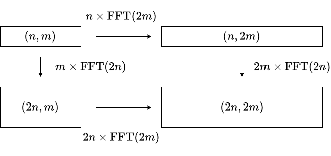
As shown in the figure above, there is a difference in computational complexity between the two calculation methods, $n\mathrm{FFT}(2m)-m\mathrm{FFT}(2n)$. Assuming $\mathrm{FFT}(n)$ is estimated to be a constant multiple of $n\log n$, it is believed that processing the FFT in the longer direction first would be faster (Nachia’s idea).
- There are frequent computations that involve performing operations on all columns of a two-dimensional array (or on every $k$-th element from a one-dimensional array). Generalizing the implementation of FFT to accommodate such cases may reduce the number of memory transfers and potentially lead to speedups.
- In the implementation introduced in this article, we always maintain values that have undergone Fourier transforms in the $y$ direction. Additionally, there’s also the possibility of maintaining values that have undergone Fourier transforms in the $x$ direction. I considered this approach as well, but I couldn’t reduce the computational complexity significantly (it remains comparable).
We have introduced several implementations so far, but it’s important to note that the efficiency improvements achieved by leveraging the properties of the Fourier transform depend on the properties of the coefficient ring, particularly the ability to perform FFT on polynomials. For those considering its use in competitive programming, it’s worth noting that an implementation may work under one modulus (e.g., $\mod 998244353$) but not under another (e.g., $\mod 1000000007$). For implementations that only involve convolution, like the one introduced initially, as long as convolution is feasible in the coefficient ring, it’s relatively straightforward to utilize.